Geospatial Data Pipelines on Vector Data often come with specific optimization challenges. The most frequent ones are point-in-polygon, spatial distance join or k-nearest neighbor. These operations, while crucial for many data science and analytical tasks, can be compute intensive, especially when dealing with large-scale datasets.
For geospatial data engineers, there are options to choose between native ST_functions in Databricks Geospatial SQL, which provide maximized precision, and grid-index systems, such as Uber’s H3 (available in Databricks as well), which enable reducing the problem to a regular column value match in a reduced dataset, sacrificing precision and putting us in risk to false negatives and false positives. There are contexts where such risk can be assumed, nevertheless… Why to choose when you don’t need to, you can have the best of both worlds: a very precise analysis and a very fast and cheap execution, compared to naive approaches.
The Precision-Latency Paradox
Geospatial engineers at mid-to-large tech companies are often trapped in a compromise between two suboptimal poles:
1. Native ST Functions
Databricks Geospatial SQL offers a rich set of native ST functions, giving developers high-precision calculations. The trade-off for this precision, however, is often performance, as full ST joins resort to resource-intensive cross-joins, even given Databricks Geospatial SQL is the best in market.
2. Index Systems (e.g., H3)
Index systems like Uber's H3 approach optimization by sacrificing precision. By converting complex geometries into a simpler, indexed format (a regular column value), the problem of a costly spatial join is reduced to a fast column value match (in a smaller dataset sometimes). This significantly increases performance compared to the full ST approach but introduces a precision compromise.
We have architected a path that ignores this false dichotomy. By treating geospatial optimization as a system-level engineering challenge rather than a simple tooling choice, we deliver full-precision analysis with "indexed" performance.
The Hybrid, Full-Precision Optimization
Without resorting to any third-party tools we can leverage Databricks' Delta Lake features, specifically ZORDER and data skipping, to create a filtered version of the full cross-join.
This is not the first post of this nature, actually this post from 2022 describes a similar approach, combining H3 and native ST_Functions to solve one particular problem, the point-in-polygon classic problem. That one consists in H3 grid-indexing through Mosaic tessellation, covering the polygonal datasets, including boundaries and splitting.
Factored has developed a new approach to handle performance bottlenecks when dealing with US country wide geospatial analysis.
- Our approach goes beyond solving point-in-polygon, it solves spatial distance join or k-nearest neighbor, and provides distance values within a given threshold R without any further compute steps after getting the solution id-pairs.
- It can be extended to any kind of input geometries, not only points and polygons,it can even work for mixed geometries in dataset A and dataset B under the same EPSG.
As an example, Factored has proposed the problem of accessibility to educational campuses/buildings through non-vehicle roads, such as bicycle roads, pedestrian roads, etc. We have to convert it into an actual measurable question under a framework:
- Given the North America Section from Open Street Map dataset, find out for each educational building, find out if it has a non-vehicle road around it under a 100m (328ft) threshold, and if it does, provide the minimum distance.
The technical problem.
- Framework: We’re using one single source of truth, which is the OSM North America session, it has tags that allow us to identify schools, universities, campuses, etc. It also allows us to identify roads and the kind of roads. Though it’s not 100% up to date, that will be our source of truth. We will derive dataset A and dataset B from the same source of truth.
- Dataset A: Educational Buildings in OSM North America
- Dataset B: Non-Vehicle Roads OSM in North America
- Geospatial Use Case: This is the classic Distance-Join with explicit distance measurement.
- Threshold: R=100m
- Outputs: Table/Report with Building Name,Building ID, Road Name (if exists), Road ID, Precise Distance.
Implementation Details
1. Prepare Geospatial Tables: The initial step involves defining and persisting geom tables, filter out bad geometries and provide a HK for each row, this will allow SQL statements to be performed on the basis of normalized ids. These tables must include latitude and longitude columns, and all coordinates should be standardized to a single EPSG. This relies on UC, Delta Lake and Databricks Spatial SQL. For strategies on how to get huge non-partitioned Datasets into UC tables efficiently. Stay tuned for another Factored.ai article coming in April.
Tables we’re going to define:
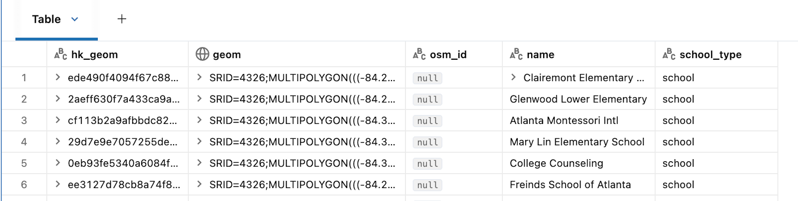
- schools: This delta table will store the multi-polygon geometries for all of the educational institutions (campuses, etc) in native geospatial databricks types, along with our identifier HK_GEOM and osm properties like osm_id and name (of the school).
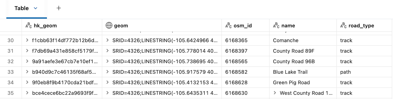
- non_car_roads: This delta table will store the multi-line geometries for all of the non-car roads (campuses, etc) in native geospatial databricks types, along with our identifier HK_GEOM and osm properties like osm_id.
2. Buffer your Dataset A: Next, buffer the geometries from dataset A using the specified threshold, R. This operation is performed using ST Functions available in Databricks Spatial SQL.
3. Grid Index and explode: The challenge in this step corresponds to finding a good resolution. That will depend on the size of the dataset maps, generally we’ve found that resolution 10 works very well for this case and for continental level cases, we’ve found this value thanks to the experience in other problems. For a very fine grained local problem(county level), you might want to choose a finer resolution. The key technology here is Uber's H3 index Functions, available in native Databricks.
In this particular use case you can replace the composite expression explode(h3_coverash3(...)) with GRID_tessellateexplode, which is the function used in the quoted article, but in our use case we don’t need the ‘is_core’ column, which is one of the computed outputs of the GRID_tessellateexplode function, this might result in an unnecessary overhead, this, we use the simpler h3_coverash3 and the native spark explode function.
The indexation of roads was shown before is a straightforward code. On the other hand, Dataset A needs to be buffered before, so edge cases are covered.
4. Optimize both datasets ZORDER-ing by each cell id: To enable efficient data skipping and clustering, optimize both datasets by using Delta Lake's ZORDER feature, based on the H3 indexes (each cell ID). This step utilizes Delta Lake ZORDER.
5. Put close geometries together (cell-id matches): Create a new dataset, D, by joining Datasets A and B on the cell-id. This guarantees that only geometries that are spatially close are paired, effectively creating a filtered subset of a cross join. This uses Databricks SQLPhoton.
6. Full Precision Join: Finally, perform the precise spatial function join (e.g., ST_Contains or ST_Distance) only on the pre-filtered subset of data (dataset D). This last step again uses ST Functions.


The result is a highly performant geospatial data pipeline that retains the accuracy required for sophisticated analytics. We’ll provide a cost/time-based benchmark across varying cluster sizes, dataset sizes, and single on hybrid-vs-native approaches.
The definition of Non-car roads for this consists in all of the Lines/Multilines in the referenced OSM dataset having the highway tag and not having a list of specific car road tag values, as provided in the definition of Dataset B. The OSM dataset along its tags is the source of truth for this experiment.
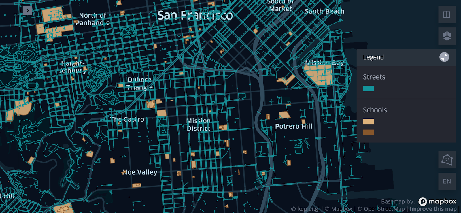
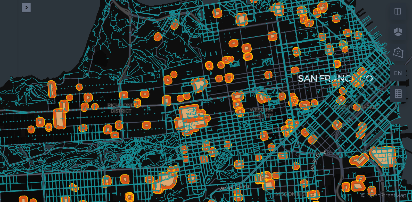
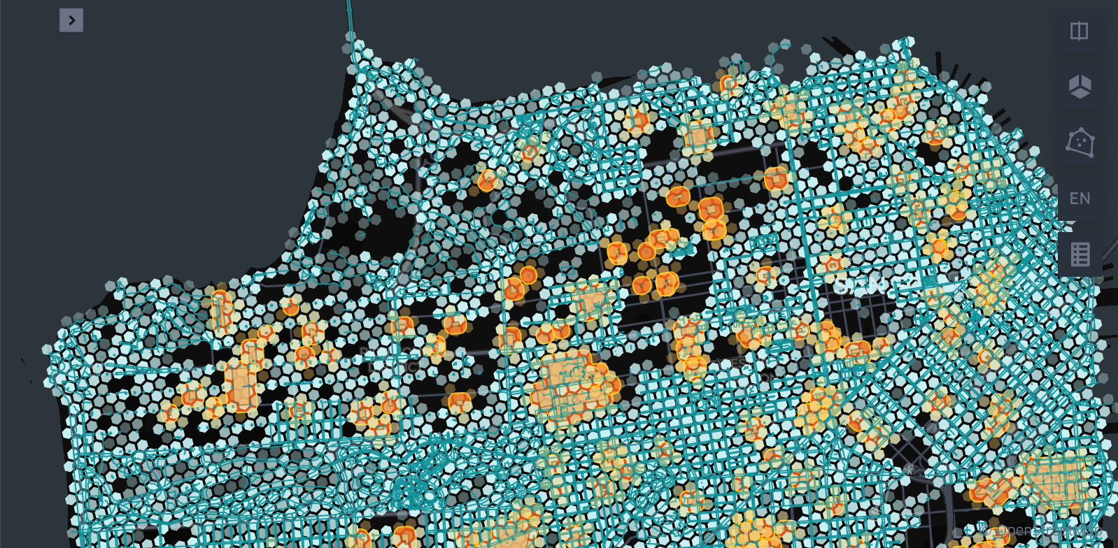
Visualizing spatial data layout
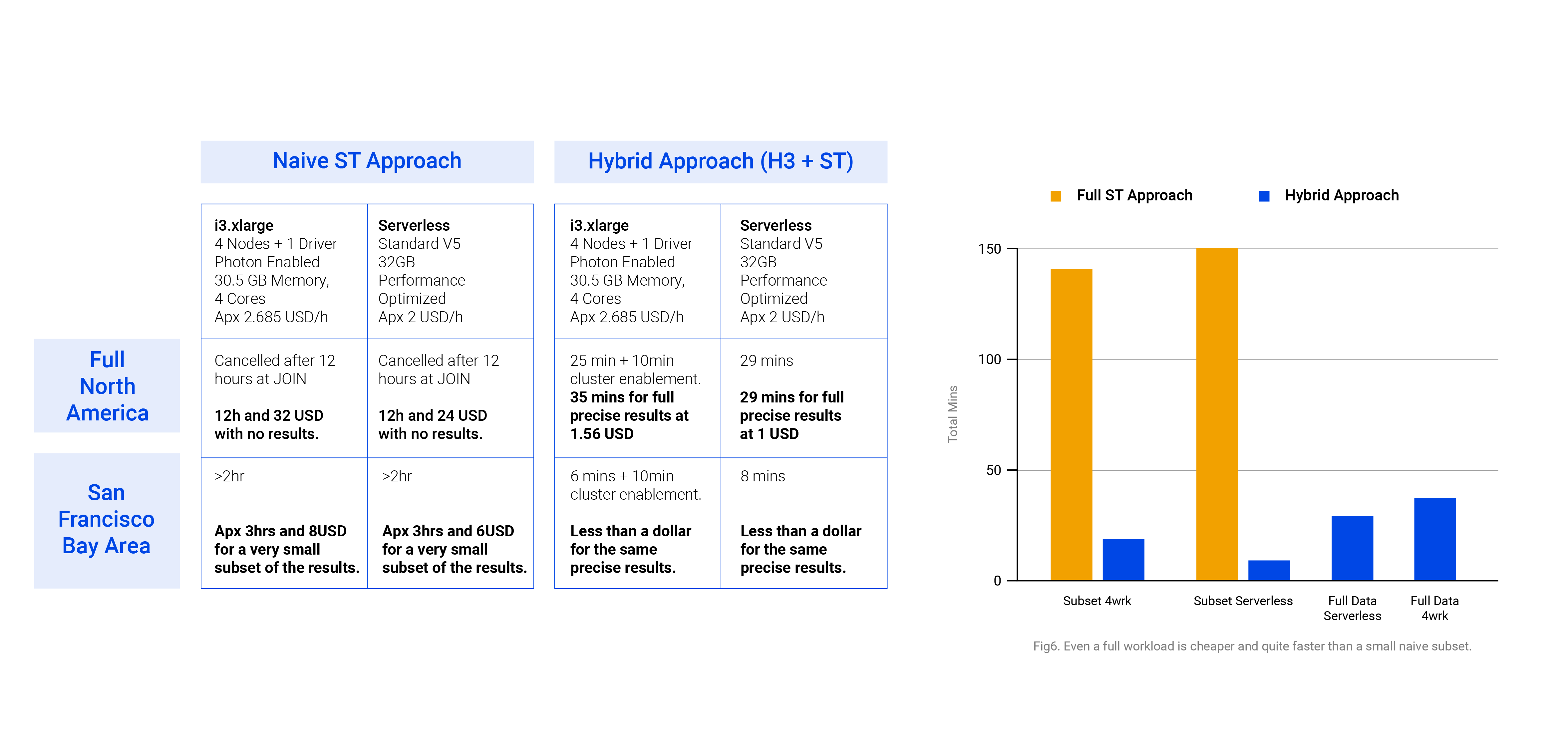
Benchmark
Considering variations in the size of the input datasets. As a prerequisite, the cluster runtime must be 17.x or greater. The current benchmark was computed on 17.3 LTS clusters. The job-cluster run was fully run on On-Demand instances with Databricks Photon Engine with the following specs:
i3.xlarge
4 Nodes + 1 Driver
Photon Enabled
30.5 GB Memory, 4 Cores
AWS is the cloud provider in this scenario. Having said that, we consider the DBU/h price at 0.15 USD and EC2 price for On-Demand i3.xlarge at 0.312 USD/h. Which means the total hourly price for our 5 nodes stands at approximately:
5*0.312usd/h+5*(0.15usd/dbu*1.5 dbu/h)=2.685usd/h
In contrast, our serverless computer with Performance Optimized (for instant start) is provided with 32GB in a Standard V5 environment. Which means around 4 DBU/h at a 0.5 USD per DBU rate. So, our hourly price stands at approximately:
0.5usd/dbu*4dbu/h=2/h
Which becomes a huge difference at intensive workflows.
In the example we were able to quickly deliver a whole data product from a formerly challenging geospatial operation: After processing and providing results at a continent level in a matter of less than one hour using a hybrid approach in Databricks Geospatial, Kepler.gl provides an interface to visually embed your cartographic solution in a website. As further work, we might experiment embedding it using Databricks Apps, for a future article.
Factored can deliver custom work like this from fast ingestions to delivering geospatial data products on Databricks apps.
Want to learn more? Schedule a call with a solutions engineer.